JSF 2.0 - "Hello World" in Eclipse (with *.xhtml pages)

Note: below description uses Eclipse Indigo, Tomcat 7.0.28 and MyFaces 2.1.7.

Requirements:

• installed Java (description here)
• installed and configured Eclipse (description here)
• installed and configured Tomcat for the Eclipse (description here)

You will learn:

• how to create "Hello World" application in JSF 2.0 using Eclipse

Note 1: The following post and example show classic JSF 2.0 application with a view technology as .xhtml pages. I do not use any additional libraries and extensions for the standard JSF libraries. I don't use (for the time being) templates. JSF implementation used comes from MyFaces.

Note 2: I use standard capabilities of IDE platform to generate the project, without those thousands automated plugins which do everything for the user. Sometimes configuration and usage of a plugin is a "pain in the ..." - in my opinion it is worth to know how to deal with a standard set of tools, and after that there is always a time to faciliate our life ;-)

In this post I will show how to create sample JSF 2.0 application using Eclipse. It will be similar application like in the post about creating sample JSF 1.2 application. But there will be some small differences, especially during generating the project and adding JSF capabilities to it. Let's do it.

Step 1: create new dynamic web project for the Tomcat. It is available in "web" menu section under option "File->New->Project":

Press "Next" to go further and set some basic project's properties:

Step 2: adding JSF capabilities for the generated project (JSF and JSTL libraries).

This step is the same as step 2 in previous JSF 1.2 example under Eclipse. Just copy all necessary .jar libraries into WebContent\WEB-INF\lib directory.

Also here there is a possibility to use Code Assist for *.xhtml pages. Unfortunately there is one difference comparing to support for JSF 1.2.x - You can click on bean/field only when Your beans are directly declared in faces-config.xml file. If Your beans are declared with the help of annotations, it does not work. This is Eclipse bug (see for example https://bugs.eclipse.org/bugs/show_bug.cgi?id=323709). It is still not fixed in Indigo, despite the fact that it should work in 3.4.x, as noted in the bug.

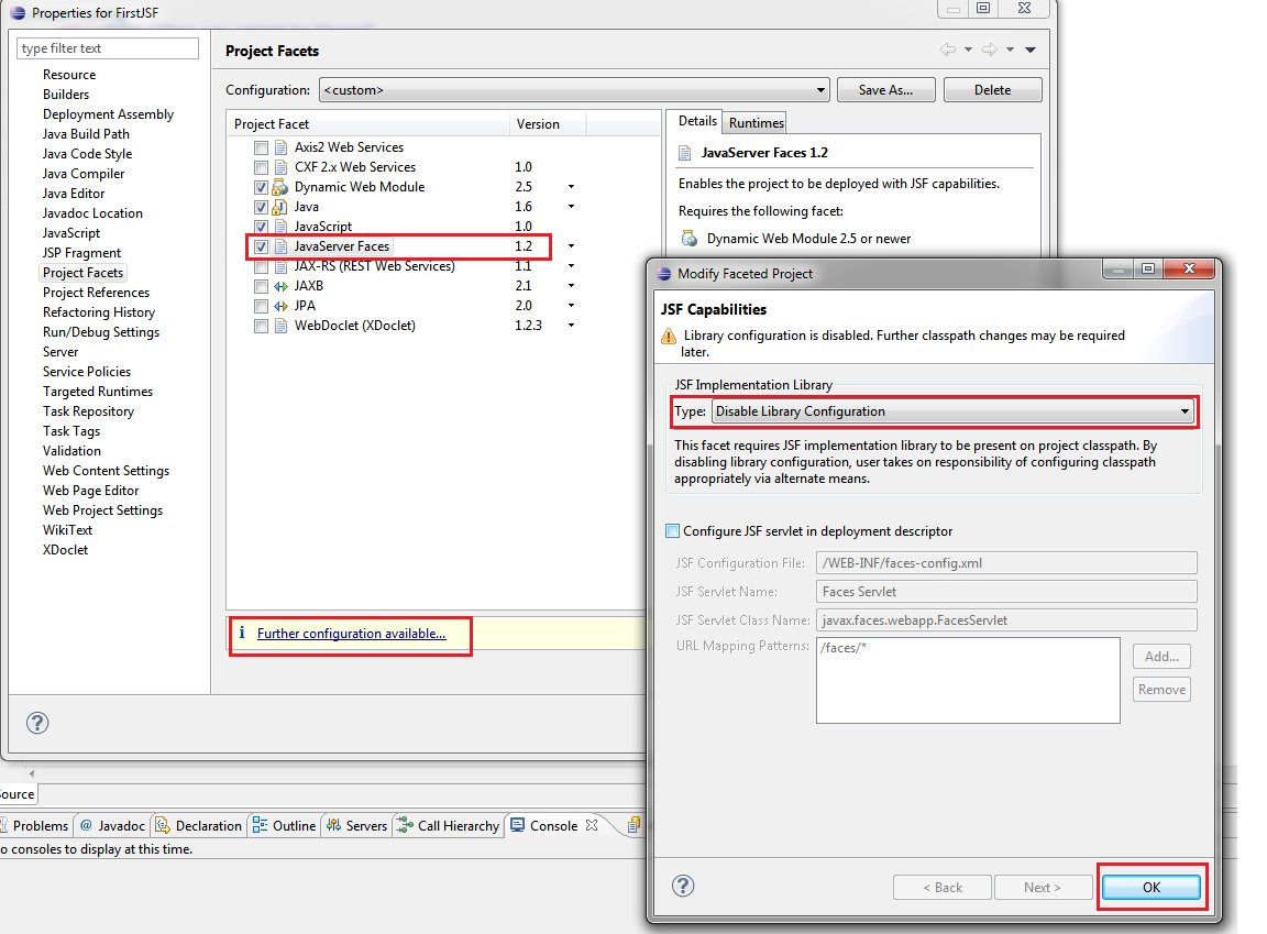
In order to enable Code Assist just open context menu and choose "Properties" option. Locate the section "Project Facets" and check the option "JavaServer Faces". Then "Further configuration available...". On the screen You have to select "Disable library configuration" and press OK:

Step 3: the project structure is ready. Creating sample application.

This will be the same application as for version 1.2 with some differences coming from JSF 2.0:

- pages extenstion will be .xhtml instead of .jsp

- we use annotations in backing beans

- there will be no faces-config.xml file (now)

Everything should look like this:

File web.xml has to be changed like shown on screenshot below:

Step 4: deployment and running.

This step is similar to steps 6 and 7 from JSF 1.2 version. After deploying application on the server and starting the server, we have to open a browser and type in URL:

http://localhost:8080/FirstJSF2

That's all. We should have working JSF 2.0 application.

-------------------------------------------

Download source files:

Note: make sure that Java, Eclipse and Tomcat are properly installed and configured for running the project (additional configuration may be required if different directories are used).

Eclipse complete sample project is here (with all required libraries). You can also download a war file located here (just copy it inside webapps folder in Your Tomcat and start Tomcat with the script startup.bat)

JSF 1.2 - "Hello World" in Eclipse (with *.jsp pages)

Note: below description uses Eclipse Indigo, Tomcat 7.0.28, MyFaces 1.2.12 and JSTL 1.2.1. 

Requirements:

• installed Java (description here)
• installed and configured Eclipse (description here)
• installed and configured Tomcat for the Eclipse (description here)

You will learn:

• how to create "Hello World" application in JSF 1.2 using Eclipse

Note 1: The following post and example show classic JSF 1.2 application with a view technology as .jsp pages. I do not use any additional libraries and extensions for the standard JSF libraries.

Note 2: I use standard capabilities of IDE platform to generate the project, without those thousands automated plugins which do everything for the user. Sometimes configuration and usage of a plugin is a "pain in the ..." - in my opinion it is worth to know how to deal with a standard set of tools, and after that there is always a time to faciliate our life ;-)

Many publications and tutorials about JSF (Java Server Faces) very briefly descibe the configuration of development environment for the described examples. Many times I saw such situation: after few sentences about "how amazing is JSF" there was a simple list of JSF tags with their attributes described. Or at the beginning there was an example of "Hello World" application and every line of code was described and explained.

I think that is what is missing is the lack of an example of complete project with its directory structure and an information how to create this project and deploy on the web server. I saw some examples where the project structure was shown, but for the building and deploying application user had to use Ant and type some commands. Great, but we need Ant, when we have Ant, we need to be familiar with it to write build.xml file, then we need something else and so on and so on.

This is of course OK if we want to write everything from scratch by hand. But wouldn't it better just to start our IDE, make some clicks and have a complete and working project ready for further development?

Let's see how it looks like in Eclipse IDE.

Step 1: creating dynamic web project for the Tomcat.

Open menu "File->New->Project" and in the "web" section find and choose "Dynamic Web Project" and press "Next":

 

Press "Next" to go further and set some basic project's properties:

After that we should have generated project structure for the web application.

Step 2: adding JSF capabilities for the generated project (JSF and JSTL libraries).

The easiest way is to download latest libraries of MyFaces 1.2.x from here and JSTL 1.2.x from here, and copy all .jar files into generated WebContent\WEB-INF\lib directory. After that just refresh the whole project by pressing "F5" on the project's root and all libraries should appear in the section named "Web App Libraries" in the project's structure.

In addition it is worth to enable nice feature named Code Assist. Code Assist allows automatically complete JSF tags when typying by pressing CTRL + Space. It also provides direct access to beans, their methods or fields directly from JSP page - just by click on bean/field name. In order to do this just right click on the project and from the opened context menu choose "Properties" option. Locate the section "Project Facets" and check the option "JavaServer Faces". Then "Further configuration available...". On the screen You have to select "Disable library configuration" and press OK:

Note: project facet "JavaServer Faces" allows to download JSF libraries automatically and add them to the project. Unfortunately JSTL libraries still needs to be downloaded manually.

Step 3: the overview of a project.

When steps 1-2 where done as described, the project structure should look like this:

Step 4: "Hello World" application.

Now we are ready to implement some sample JSF application. First we should create a package named com.firstjsf.backingbeans in the "src" directory. Second we should create two classes inside the package named HelloMessageBean and WelcomeBean. Third we should modify generated faces-config.xml file by adding there our classes and navigation rules. Everything should look like this:

Be careful about small and big letters - names should be exactly as shown above. In the faces-config.xml file we created entries for the navigation rules for not existing yet web pages. Let's create those web pages (index.jsp and message.jsp) in the WebContent directory:

Application is ready.

Step 5: deploying on Tomcat.

At the bottom of a screen locate "Severs" tab. We should have already Tomcat there. Right click on server name to open its context menu, ten choose option "Add and Remove...":

Choose our project and add it to the server by pressing "Add" button:

Step 6: running the application.

Go back to the "Server" tab again and make sure that our project is visible on the server. Then click the marked icon to start the server:

After starting the server we should see that the server state was changed:

After deploying application on the server and starting the server, we have to open a browser and type in URL:

http://localhost:8080/FirstJSF

What next? This simple working project can be used as a base for further learning about JSF. For example we can change the view technology from .jsp to facelets. We can add libraries which extend our standard tags by adding tags with ajax support, i.e RichFaces.

-------------------------------------------

Download source files:

Note: make sure that Java, Eclipse and Tomcat are properly installed and configured for running the project (additional configuration may be required if different directories are used).

Eclipse complete sample project is here. External libraries folder (with JSF and JSTL) is here. You can also download a war file located here (just copy it inside webapps folder in Your Tomcat and start Tomcat with the script startup.bat)

"My databse is slow" - part 3: some technical stuff

Note: below description uses PostgreSQL 8.3.7.

In the previous two articles I tried to show what can affect the overall performance of the database and how important are indexes.

If we assume that the database is normalized, memory settings for the server are ok and we have indexes, the only way to check the performance is monitoring the query plans. Therefore I would like to return once again to the query plans and look at them with more details.

From the previous post, we know that we can generate plans for queries using two commands. These commands are:

• EXPLAIN SQL_command
• EXPLAIN ANALYZE SQL_command - this command is a variant of the first with small difference: examined query is executed and EXPLAIN ANALYZE returns the real execuion time.

Using the test database from the previous post, let's see the query plan for the following SQL command:

select * from customers where lname = 'Cervantes';

To see the query plan, execute those two commands:

vacuum analyze;
explain select * from customers where lname = 'Cervantes';

Query plan that has been generated for this query is as follows:

Always we are most interested in "the highest" line of displayed plan - it shows the total cost of the query execution, after all other internal operations for more complex queries (eg joins, sorts, etc.).

In our case we have: (cost: 4.51 .. 59.47 rows = 33 width = 18). What does it mean?

1. cost: 4.51 .. 59.47 - this is an interval defining total execution time measured in special units called disk page fetches - these units are not seconds nor other units of time. First number estimates time needed to retrieve first row in the result, second estimates total cost of returning all rows in the result. The calculation of this value is "higher mathematics", especially if the query uses more techniques than primitive table sequential scanning - which is the easiest and can be easily calculated. Unfortunately, but only for primitive examples like "select * from some_table" (without the use of indices to be 100% sure that the scan will be performed sequentially and without any query conditions "where"), You can find over the Web some examples of calculating these values. Those who are interested in more details and technical stuff, should visit this page
2. rows = 33 - this is estimated number of rows returned by a query.
3. width = 18 - this is estimated size (in bytes) of all the returned rows

Above data are obtained on the basis of statistics located in a special system tables. There are two tables of statistics which are crucial for the query planner:

1. pg_class - contains information about certain database relations (tables, indexes, etc.), i.e. their location and size.
2. pg_stats - contains information about the data stored in tables, i.e. the most common values, the frequency of common values occurrence.

Let's see what are the statistics for the table "customers", and what is their impact on some elements of the query plan for above query about user "Cervantes".

Returned data mean that the table "cutomers" has 10.000 records and is located on 62 "pages".

Returned data are based on some statistical data for all the columns in the table "cusotmers" and their content. It is specified which values are most popular, what is their frequency, and amount of values which are different from each other.

What is the meaning of this data in the context of our query about "Cervantes" user?

pg_class - is the basis in calculating the cost of the query execution. For our "Cervantes" query  in the case of sequential scan (if there were no index on the "lname" field in the Customers table), we would calculate the cost from the formula:

(relpages * SEQ_PAGE_COST) + (reltuples * CPU_TUPLE_COST) + (relpages * CPU_OPERATOR_COST)

Capitalized names are costs of arbitrary operation - the are defined in postgresql.conf. Unfortunately (or "fortunately"), our query uses indexes, so the calculation of the cost is a bit more complicated (task for volunteers, formulas are here, You only have to to be familiar with the concepts of "last recently used buffers" (LRU) and Mackert-Lohman formula ;-)).

pg_stats - allows to estimate the number of rows returned in a query using given logical condition (in our case: "where lname = 'Cervantes'"). In our case for the "Cervantes" query we are lucky - "Cervantes" occurs directly in the list of most common surnames, and also is known for its occurrence. The number of rows returned is calculated using the formula:

relpages * selectivity

where:

selectivity = most_common_freqs["Cervantes"]

Hence we get:

10000 * 0,00333333 = 33

And what if we are looking for value which is not in the column "most_common_freqs"? Then the formula has a different form:

selectivity = (1 - sum(most_common_freqs))/(num_distinct - num_most_common_vals)

Calculating selectivity value for the name "Smith", I leave for volunteers as usually ;-). Remember that first You have to execute "vacuum analyze" and then view statistics and then the query plan.

-------------------------------------------- 

Some notes about the statistics:

The content of statistics tables is generated based on random samples taken from the tables in the database. Generating (and therefore refreshing) full statistics takes place during the execution of the VACUUM ANALYZE command. Hence, it is very important to run this command periodically to ensure that statistics for the planner are up to date. Therefore, before showing the above example the first command executed by me was VACUUM ANALYZE in order to query plan be based on the most reliable statistics.

It should be noted that next execution of this command can generate a slightly different statistics, so query plan for the same query may be slightly different (in terms of cost and estimated number of rows). This is because of mentioned random samples taken for calculations.

--------------------------------------------

A few final notes about performance

I can say that the general rule to optimize query execution time is as follows:

"There is no certain way to increase performance in all cases. The best method is trial and error."

In practice it means to try to generate different query plans (in addition to that which is generated by default) and select those with the best execution time. These attempts usually involve forcing the query planner  to behave in different way which leads to a different query plan. This can be achieved through:

1. Forcing the query planner to use an index (often the index exists but is not used by the planner). This can be done for example by:

• switching off a global sequential scans by setting enable_seqscan = off in postgresql.conf file
• partial indexes (conditional) - You can create a conditional index for the most frequently returned data in column
• indexes using multiple fields (watch out for the order - the order of fields in the index should be the same as the order of fields in queries)
• some SQL tricks related to change the query selectivity, for example using LIMIT, ORDER BY or trailing condition AND TABLE_ID = TABLE_ID (where TABLE_ID is a master key in the table)

2. Changing the order of joining multiple tables, for example executing "(A join B) join C" can be different than executing "A join (B join C)" - this is similar to a problem of  "optmial matrix-chain multiplication".
3. Using stored procedures, views, breaking huge query into a number of smaller queries .

Interesting fact (found over the Web):

In order to monitor the progress of executing a long query to the database (a really long time, not a few seconds) you can create a sequence with the value set to 1 (eg, the sequence "monitor_seq") and add it to executing query:

select nextval('monitor_seq'), column1, column2....

Executing:

select currval('monitor_seq');

at the time of running the long query will show us the progress.

"My database is slow" - part 2: indexes.

Note: below description uses PostgreSQL 8.3.7.

This article is a continuation of previous one about database performance.

Suppose we have a database that is normalized to our needs, the memory of the server was also quite reasonably allocated, we are using a connection pool and we did not change the default transaction isolation level for our database - but the database still is not a "speed daemon". What can You do in this situation? Did we miss something?

You can look inside the database giva a closer look on specific operations performed on the data to determine which operations cause performance degradation and possibly "help" them perform faster. As the sample database I will use PostgreSQL - I will examine its specific mechanisms to check and improve performance. This will be only an outline of what can be done (based on crude example), because the topic is so large that it may well be placed on a separate dedicated blog.

Requirements:

• installed PostgreSQL (description here)
• a test database with sample data - just to show how PostgreSQL performs a very simple SQL opeartions

Let's consider a very simple database for some online store with two tables: customer table (called Customer) and customers' orders table (called Order). Just open pgAdmin and execute this SQL command:

CREATE DATABASE store ENCODING = 'UTF8';

Then connect to database "store" and run this SQL commands:

CREATE TABLE customers
(
customer_id INTEGER,    
fname VARCHAR(32),
lname VARCHAR(32) NOT NULL,
CONSTRAINT customer_pk PRIMARY KEY(customer_id)
);

CREATE TABLE orders
(
order_id INTEGER,
customer_id INTEGRE NOT NULL CONSTRAINT customer_order_fk REFERENCES customers(customer_id),
description TEXT,
price NUMERIC(7,2),    
CONSTRAINT order_pk PRIMARY KEY(order_id)    
);

For simplicity, here I do not use a SERIAL field to hold primary keys - just ordinary integer with constraint. Now we should fill the database with some sample data: lets put about 10 000 records to Customers table and 30 000 records to Orders table.  That is rather huge amount of data. How can we do it?

The best way is to write a Java program that generates a file with proper SQL INSERT statements for each table - this is homework for You ;-)

I wrote simple program which takes popular first names for males and popular first names for females, then takes popular surnames from here and combines them together to produce 10.000 "people". Having those records and knowing their customer_id (that's why I used ordinary integer field - just to write a program) my program generated random 30 000 orders for those customers.

And now suppose we want to retrieve all customers named Smith and we want to see all orders for each customer Smith. We need two queries:

select * from customers where lname = 'Smith';
select * from orders join customers on orders.customer_id=customers.customer_id where customers.lname = 'Smith';

In my case, the first query returns just 9 customers named Smith (from total of 10 000) and 30 orders (from total of 30 000) for all 9 "Smiths".

Okay, we have SQL commands - but how can we check their execution time on a database? PostgreSQL provides two commands that show details about executed commands:

a) EXPLAIN SQL_command

b) EXPLAIN ANALYZE SQL_command - this command is a variant of the first with small difference: examined query is executed and EXPLAIN ANALYZE returns the real execuion time.

Before we show an example of above commands execution, some technical information about the process of executing the query by PostgreSQL: when the PostgreSQL server receives SQL command from client application, the query string is passed to the query parser that checks for syntax errors. If everything is ok, parser based on the query creates a structure called the query tree. Then, this structure is passed to the query planner which generates all possible query plans and chooses the shortest one from them. This plan is passed to the executor who performs the query and returns the records in the manner described in query plan.

Mentioned EXPLAIN command displays the details of the plan chosen by the planner as the shortest one. Let's see the result of executing EXPLAIN ANALYZE for the queries about users Smith:

Because reading query plans and their details is a separate art, we will focus on the actual run time (visible as a Total Runtime, respectively 1,482 ms for the first question, and 16,552 ms for the second question).

Lets provide indexes for the fields we are searching for and for the fields where the join operation is performed. In our case it will be:

a) the lname column of the Customers table - create index with the command: 

CREATE INDEX lname_index ON customers USING btree (lname);

b) the foreign key column in Orders table (the column cutomer_id) - create an index using the command: 

CREATE INDEX customer_fk_index ON orders USING btree (customer_id);

Note:

After You create indexes, You have to refresh the statistics used by database planner to calculate the optimal query plan. This is done by running VACUUM ANALYZE command. After executing this command, once again execute the EXPLAIN ANALYZE command for our "Smith" queries:

 

The results of the queries which are several times faster than previously. They are respectively: 0,123 ms (1,482 ms previously), and 0,507 ms (16,552 ms previously).

The advantage is obvious. But whether the index will solve all our problems? Not always. There is no guarantee that the planner will benefit from the index. Sometimes it appears that the sequential table scan can be faster than using an index (such behavior may depend on the "selectivity" degree of certain query). In most cases it is good to have indexes - they can only help.

"My database is slow" - part 1

Note: below description uses PostgreSQL 8.3.7.

Perhaps You often heard complaints that some application is veeeery sloooow. Despite the technology used, bought another X GB of RAM and so on the problem still exists. Sometimes the cause can be very simple - interaction with the database can be a bottleneck and a source of all problems. This can be checked and possibly improved.

Often the developer itself must change something in the database - do not be afraid to say it - hire a database magician cost a lot of money for the company and often the developer becomes a database specialist ;-). Therefore, anyone who changes something in the database must have some knowledge. Otherwise, some ad-hoc changes can cause a lot of performance problems.

What can you do then? Having the database, You can take a closer look on some points:

1. Database normalization (decomposition).

Simply said - making a database to be in the n-th normal form. You may naively believe that "the database engine can handle" somehow our SQL query, without worrying ourselves about performance. Theoretically yes, even nightmarish database schema will work somehow - after all, a bit smarter (than the rest) people formed the principles of relational databases. The problem starts when our application is no longer a primitive data browser which executes the same "select" SQL query all the time. That's why the other smarter people have invented a normalization. For example this allows the database engine not to retrieve 20 columns from one table just to show us only those 2 which we are interested.

For example let's assume that we have a company and we store all the employees in a one big table:

CREATE TABLE employees ( 
id                int4 PRIMARY KEY,
active            boolean, 
first_name        varchar, 
middle_name       varchar, 
last_name         varchar, 
ssn               varchar, 
address1          varchar, 
address2          varchar, 
city              varchar, 
state             varchar(2), 
zip               varchar, 
home_phone        varchar, 
work_phone        varchar, 
cell_phone        varchar, 
fax_phone         varchar, 
pager_number      varchar, 
business_email    varchar, 
personal_email    varchar, 
salary            int4, 
vacation_days     int2, 
sick_days         int2, 
employee_number   int4, 
office_addr_1     varchar,
office_addr_2     varchar, 
office_city       varchar, 
office_state      varchar(2), 
office_zip        varchar, 
department        varchar,
title             varchar,
supervisor_id     int4
); 

And now some Secretary wants to find those people who earn more than 5000 USD:

SELECT first_name, last_name from employees where salary > 5000 ;

Let's assume that the company is a big corporation which employs thousands of people. Database engine must scan entire table, retrieve all columns for people who earn more than 5000 and at the end pefrorm a projection and return only 2 columns - first name and last name.

Note: do not kid ourselves - normalization is not an ideal remedy for performance problems, and sometimes may even contribute to decrease a performance. Why? For example let's take huge reporting queries that collect a lot of cross-sectional data. In the fully normalized database, the amount of join operations between tables can be very large and could have significant impact on performance. Sometimes it is better to have non-normalized parts of database schema, or even have non-normalized redundant data tables (for generating reports) next to normalized parts. There is no silver bullet solution for that - the approach depends on specific problem. 

2. Memory configuration for the server.  

The fact that Your hardware allows You to play latest games, does not mean that the database will work fast. Even 10-th normal form of a database schema and super-optimal queries will not help when server has total memory similar to required by old DOS games. Sooner or later because of lack of memory many I/O disk operation will be performed to compensate memory request. System resources are important. Unfortunately, at this point databases vary widely in terms of available configuration options. "No silver bullet" also applies here - the only way to discover best performance is to tune database memory settings and test it against SQL queries. 

3. Opening connection to the database.

Although the authors of JDBC drivers maintain that connection cost is small and well optimized, we must not forget that after all this is some expense. As an example, consider a typical web application where in every moment a user clicks on different screens, which show him various data. We have to approaches here:

• maintaining an open connection during user's working time
• opening connection for each request, performing some database query, returns the result (which is presented to the user) and closing the connection.

First approach is expensive (in terms of resources and performance), second is much better. But when we take into account the large number of users and their actions, total cost of opening and closing connections may have considerable importance. It is worth here to consider using the so-called connection pool - such as Apache DBCP or C3P0. Responsibility for creating/closing of connections goes to connection pool. The pool itself has various configuration options that can increase the efficiency of cooperation with the database application. For example some connections may have been opened after startup and ready to immediate use and so on. 

4. Transaction isolation levels and locks.

Transaction isolation levels have a direct impact on the types of locks used. If You are not sure how to choose the level of transaction isolation, it is better to remain at the default level for a particular database. You have to remember one important thing: the higher isolation level you choose the more subtle and complex lock must be use by the database engine to provide concurrent access to data. Using higher levels of isolation can also cause deadlock occurrence.

Note: You may not agree with mentioned points. They are only my personal subjective choice based on problems and observations during my work. Database performance is a very broad issue dependent on many factors - I pointed only four general issues, but You may find another four or more which will be just as important and necessary.

Installing and configuring Tomcat for Eclipse

Note: below description uses Tomcat 7.0.40.

Probably You always wanted to write your own web-based application in Java (ok, read: writing another Facebook-like portal and live in luxury in Dubai to the end of Your life ;-)). Of course it is possible, but before that inevitable moment occurs, You have to do much more simple thing - configure the environment for developing web applications (unless You are headmaster in Your own company and someone else does it for you...).

So let's look at how to configure Apache Tomcat which is professionally defined as the servlet container (i.e. for JSP). I will show how to configure it under Eclipse.

Recall that so far we have managed to install Java and set up Eclipse to work with it. It is time for Tomcat. 

Step 1: download the Tomcat binary distribution (core version as a .zip file) from here

Step 2: Unpack the .zip from step 1 to the C:\Development\Tomcat directory. We should get something like this:

Step 3: Open Eclipse IDE and the Java EE perspective (Window menu -> Open Perspective -> Other -> Java EE). This will be the default perspective for our work. Using this perspective, at the bottom in the "Servers" tab we add a new server:

Step 4: Configure the new server. Select the type of the server (Tomcat 7) and leave the name set to localhost:

Step 5: Further configuration of the new server. Select the server's installation directory (in our case C:\Development\Tomcat) and Java virtual machine which will be used - in this case it will be the same virtual machine which we configured to work with Eclipse (see this article).

After pressing Next, Eclipse will display a window asking You to add some web applications to the newly defined server. Ignore this by pressing Finish.

Step 6: Basic configuration of a server. Open server configuration panel by double click on the server name on Servers tab.

We allow the Eclipse to manage Tomcat installation and use wtpwebapps  folder (in Tomcat directory structure) for deploying our applications. In addition we change the way Tomcat publish applications on the server - each application will have a separate xml configuration file in Tomcat (so-called "context" file).

Tomcat is ready and configured to work. We can start and stop it using the icons on the right side in the "Servers" tab. The results of these operations (logs), are visible in the "Console" tab.

Installing PostgreSQL (hard version)

Note: below description uses PostgreSQL 8.3.7 version installed on 32 bit Windows XP.

In a previous article I presented how to install PostgreSQL using Windows installer. It was quite easy. But ...

There are people that do not play with such ease, what is more, they can not stand when the system is doing something for them in the background, when something is installed - some services, user accounts... They feel insecure, they are suspicious - only the execution of all activities from the command line calms their nerves.

This time, I prepared the description for the people who love technical masturbation and who love to do everything manually and have everything under control. We'll become the PostgreSQL installer and manually execute all the installation steps to get an effect similar to using Windows Installer. So, let's get to work.

Requirements:

• we are working on Windows XP using account with Administrator rights (or we belong to the Administrators group)
• database will be installed to C:\Development\PostgreSQL (the same as when using Windows Installer)
• disable all antivirus/firewall (this one from Windows too)

Step 1: download the version of the installation file (.zip) of PostgreSQL from here. Download the file with the "binaries-no-installer" part in its name.

Step 2: extract the contents of the file from step 1, to C:\Development\PostgreSQL (zip has the pgsql directory and rest of the folders inside it - I recommend to get rid of it and move all subfolders to C:\Development\PostgreSQL - we will have a shorter path). We should get something like this:

Step 3: we need to create an empty directory named "data" in the directory C:\Development\PostgreSQL (along with the rest of the directories from the picture above).

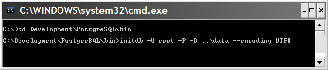
Step 4: create and initialize the database cluster (remember that we are working on the account with Administrator rights). To do this go to the console to the directory C:\Development\PostgreSQL\bin and execute the command:

Desription:

• option "-U root" means the owner of the database named root - such user account will be created in database (as a superuser)
• option "-W" means that You will be prompted for a password for this user
• option "-D .. \ data" means the location of the files for generated database
• option "- encoding = UTF8" means that the server will have UTF8 encoding by default (each newly created database too!)

After executing this command, we should see sometling like this:

At the bottom, PostgreSQL offers us to run a newly created database using two different commands. It will not work (You can execute those command to see what error is generated) - remember that we are working on account with Administrator rights, and for safety reasons, we can not start and stop the PostgreSQL server on that account. We should create a system service which will run PostgreSQL server process.

--------------------------------------------

The short version:

Step 5: Perform the following command in the console:

That's all. You're done. The service will be created and registered for the Local System Account. This is a special account which can run services, but it is not a typical account with administrator privileges (more info here).

Do not run the service yet.

--------------------------------------------

Long version:

Step 5: continue to imitate the installer. PostgreSQL installer creates a special account with no administrator privileges - so we will also create such account. Acount login and password will be both set to "postgres". We go to Computer Management, then Users:

Now we add new user with login and password postgres:

For the security reason we do not allow to change the password.

We would like now to make "postgres" account able to run the PostgreSQL server. So we need to create and register a special service for this account, which will carry out these operations. Before we do that we need to assign to this account the appropriate permissions to directories where database server is installed.

Step 6: Change the access permissions for the directory server for the postgres account.

And so:

1. Directory C:\Development should only have read permission.

2. Directory C:\Development\PostgreSQL (and its subdirectories) should have all possible permissions.

Step 7: Registering the service.

Using the console go to the directory C:\Development\PostgreSQL\bin and execute there this command:

Description:

• option -N "PostgreSQL Service" defines the service name
• option -U postgres says on what account the service is launched
• option -P postgres gives the password for service account
• option -D "C:\Development\PostgreSQL\data" tells where database cluster is located (be careful it is very important here to give the full path to the directory "data")

We do not run the service.

--------------------------------------------

Configuration:

Before starting the service must change the basic settings. Move to the directory C:\Development\PostgreSQL\database and open the file postgresql.conf. In this file, You must find and uncomment the following lines:

• listen_addresses = 'localhost'
• port = 5432

Now You can start a service in the panel management services.

If everything was done properly, the service should start. If we chose the longer version, in case of trouble with starting the service we should go to the configuration of a service, then select an account for this service and retype password for that service (in our case: postgres)

Theoretically we have the ability to log from the console to the database using the command line (marked red colour):

Thus we should get exactly the same result as using the Windows Installer.

Notes: a short way works ok under Windows XP Prof., should also works ok under Windows Vista - in both systems there is the Local System Account for services. For Windows 2000 You must perform the installation in a long way. For safety, PostgreSQL installer always chooses longer way - it creates an account for the service, then creates sevice itself and registers it to the created account.